Tutorial
from curves import Derivative Curves ======
as Identity (eye)
>>> from curves import Curve, lin
>>> eye = Curve()
>>> eye(123.456)
123.456
>>> f = eye + 5
>>> f(10)
15
>>> set(eye(x) - x  for x in lin(-5, 5))
{0}
as Constants
>>> from curves import Curve
>>> f = Curve(1) + Curve(7)
>>> f(123.456)
8
>>> f = eye + Curve(7)
>>> f(3)
10
as Functions
>>> from math import exp, pi
>>> exp = Curve(exp)
>>> exp
exp
>>> exp(1.)
2.718281828459045
such prepared functions are available as
>>> from curves import Curve, lin
>>> from curves.functions import sin, cos
>>> sin
sin
>>> f = sin ** 2 + cos ** 2
>>> f
sin ** 2 + cos ** 2
>>> f(123.456)
1.0
>>> set(round(f(x), 12) for x in lin(-pi, pi))
{1.0}
as Variables
>>> from curves import X  #  same as Curves('X')
>>> X
X
used to build polynomials
>>> p = X ** 2 + 2 * X - 3
>>> p
X ** 2 + 2 * X - 3
>>> p(1) 0>>> p(-1) -4
Compositions
>>> from math import exp, sqrt, pi, log
>>> from curves import Curve
>>> exp = Curve(exp)
>>> exp
exp
>>> X = Curve('X')
>>> X
X
>>> f = exp(X)  # same as exp @ X
>>> f
exp(X)
>>> phi = 1 / sqrt(2 * pi) * exp(-(X ** 2) / 2)  # std normal density
>>> phi(0)
0.3989422804014327
>>> phi(1)
0.24197072451914337
>>> g = exp @ log
>>> round(g(123.456), 12)
123.456
Inplace Operations
>>> from curves import X
>>> X += 2
>>> X
X + 2
>>> X(1)
3
>>> X -= 2
>>> X
X
>>> X(1)
1
>>> X -= 2
>>> X
X - 2
>>> X(1)
-1
Operators
Derivative
>>> from curves import Curve, Integral, Derivative, plotter
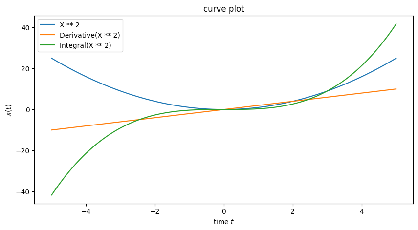
>>> f = Curve('X') ** 2
>>> df = Derivative(f)
>>> df(6)
12.0...
Integral
>>> F = Integral(f, a=0)
>>> F(6)
72.0...
>>> plotter[-5: 5](f, Derivative(f), Integral(f))
Plotting
>>> from math import sqrt, pi
>>> from curves import Curve, X, plot, lin
>>> from curves.functions import exp, sin, cos, ramp, step
>>> from curves.operators import Integral, Derivative
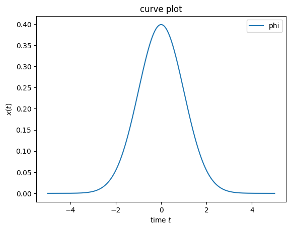
set x values
>>> x = lin(-5, 5, num=500) # x values from -1 to 1
define the function
>>> std_norm_pdf = 1 / sqrt(2 * pi) * exp(-(X ** 2) / 2)
and plot it
>>> plot(x, phi=std_norm_pdf)
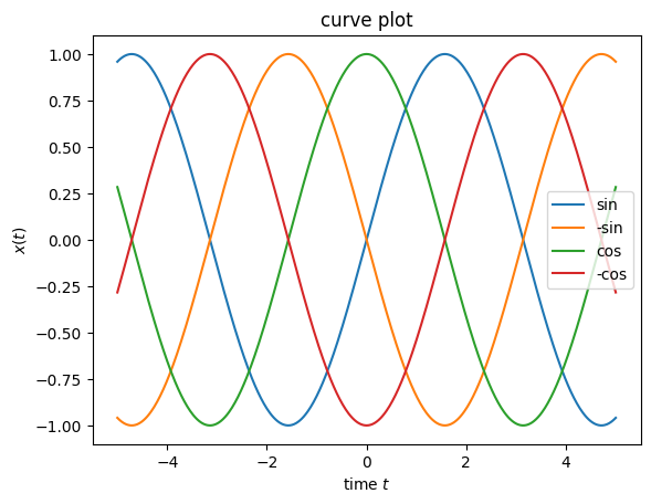
as simple as
>>> plot(x, sin, -sin, cos, -cos)
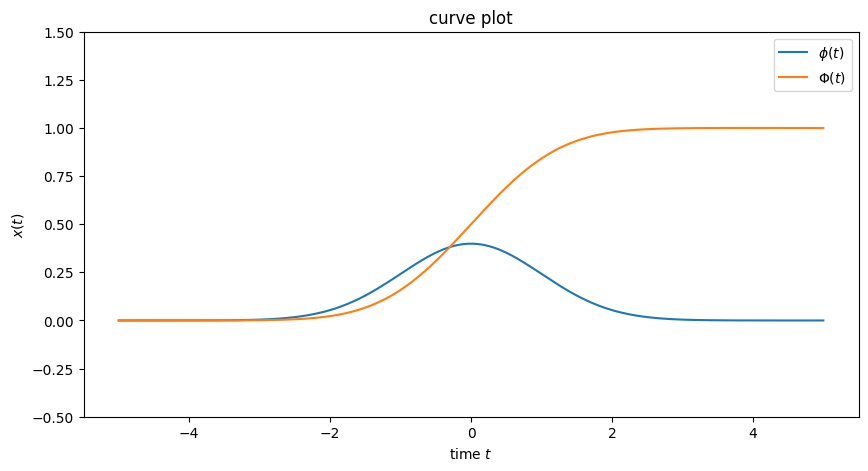
And even labels with LaTeX labels are possible
>>> curves = {r"$\phi(t)$": std_norm_pdf,
...           r"$\Phi(t)$": Integral(std_norm_pdf, -10)}
>>> plot(x, **curves, ylim=[-1/2, 3/2], figsize=(10, 5))
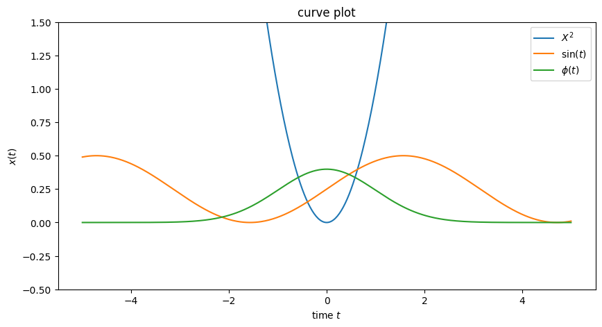
or
>>> f = X ** 2
>>> curves = {
...     r"$\phi(t)$": std_norm_pdf,
...     f"${str(f).replace(' ** ', '^')}$": f,
...     r"$\sin(t)$": (1 + sin) / 4
... }
>>> plot(x, **curves, ylim=[-1/2, 3/2], figsize=(10, 5))
and so
>>> from matplotlib import pyplot as plt
>>> x = lin(-1, 2)
>>> plt.figure(figsize=(10, 5))
>>> plt.subplot(121)
>>> plot(x, ramp, Derivative(ramp), ylim=[-1, 2], aspect=True, show=False)
>>> plt.subplot(122)
>>> plot(x, step, Integral(step), ylim=[-1, 2], aspect=True, show=False)
and so
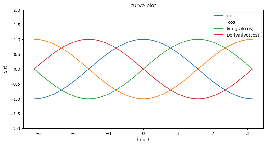
>>> x = lin(-pi, pi)
>>> plot(x, cos, -cos, Integral(cos), Derivative(cos), ylim=[-2, 2], figsize=(10, 5))